Readability formulas

Readability scores were originally developed to assist primary and secondary educators in choosing texts appropriate for particular ages and grade levels. They were then picked up by industry and the military as tools to ensure that technical documentation written in-house was not overly difficult and could be understood by the general public or by soldiers without formal schooling.

There are many readability metrics. Nearly all of them calculate some combination of characters, syllables, words, and sentences; most perform the calculation on an entire text or a section of a text; a few (like the Lexile formula) compare individual texts to scores from a larger corpus of texts to predict a readability level.

The most popular readability formulas are the Flesch and Flesch-Kincaid.

Flesch readability formula

 

Flesch-Kincaid grade level formula

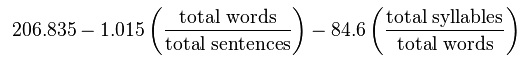
The Flesch readability formula (last chapter in the link) results in a score corresponding to reading ease/difficulty. Counterintuitively, higher scores correspond to easier texts and lower scores to harder texts. The highest (easiest) possible score tops out around 120, but there is no lower bound to the score. (Wikipedia provides examples of sentences that would result in scores of -100 and -500.)

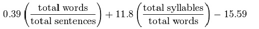
The Flesch-Kincaid grade level formula was produced for the Navy and results in a grade level score, which can be interpreted also as the number of years of education it would take to understand a text easily. The score has a lower bound in negative territory and no upper bound, though scores in the 13-20 range can be taken to indicate a college or graduate-level “grade.”

So why am I talking about readability scores?

One way to understand”distant reading” within the digital humanities is to say that it is all about adopting mathematical or statistical operations found in the social, natural/physical, or technical sciences and adapting them to the study of culturally relevant texts. E.g., Matthew Jocker’s use of the Fourier transform to control for text length; Ted Underwood’s use of cosine similarity to compare topic models; even topic models themselves, which come out of information retrieval (as do many of the methods used by distant readers); these examples could be multiplied.

Thus, I’m always on the lookout for new formulas and Python codes that might be useful for studying literature and rhetoric.

Readability scores, it turns out, have sometimes been used to study presidential rhetoric—specifically, they have been used as proxies for the “intellectual” quality of a president’s speech-writing. Most notably, Elvin T. Lim’s The Anti-Intellectual Presidency applies the Flesch and Flesch-Kincaid formulas to inaugurals and States of the Union, discovering a marked decrease in the difficulty of these speeches from the 18th to the 21st centuries; he argues that this  decrease should be understood as part and parcel of a decreasing intellectualism in the White House more broadly.

Ten seconds of Googling turned up a nice little Python library—Textstat—that offers 6 readability formulas, including Flesch and Flesch-Kincaid.

I applied these two formulas to the 8 spoken/written SotU pairs I’ve discussed in previous posts. I also applied them to all spoken vs. all written States of the Union, copied chronologically into two master files. Here are the results (S = spoken, W = Written):

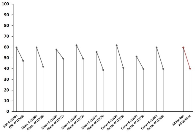
Flesch readability scores for States of the Union. Lower score = more difficult.

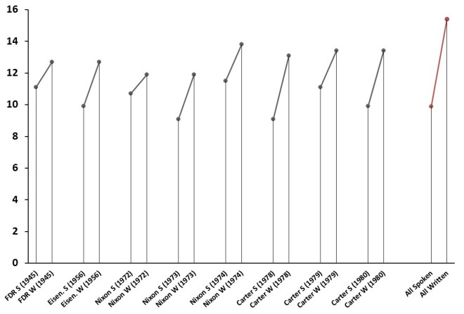
Flesch-Kincaid grade level scores for States of the Union.

The obvious trend uncovered is that written States of the Union are a bit more difficult to read than spoken ones. Contra Rule et al. (2015), this supports the thesis that medium matters when it comes to presidential address. Presidents simplify (or as Lim might say, they “dumb down”) their style when addressing the public directly; they write in a more elevated style when delivering written messages directly to Congress.

For the study of rhetoric, then, readability scores can be useful proxies for textual complexity. It’s certainly a useful proxy for my current project studying presidential rhetoric. I imagine they could be useful to the study of literature, as well, particularly to the study of the literary public and literary economics. Does “reading difficulty” correspond with sales? with popular vs. unknown authors? with canonical vs. non-canonical texts? Which genres are more “difficult” and which ones “easier”?

Of course, like all mathematical formula applied to culture, readability scores have obvious limitations.

For one, they were originally designed to gauge the readability of texts at the primary and secondary levels; even when adapted by the military and industry, they were meant to ensure that a text could be understood by people without college educations or even high school diplomas. Thus, as Begeny et al. (2013) have pointed out, these formulas tend to break down when applied to complex texts. Flesch-Kincaid grade level scores of 6 vs. 10 may be meaningful, but scores of, say, 19 vs. 25 would not be so straightforward to interpret.

Also, like most NLP algorithms, the formulas take as inputs things like characters, syllables, and sentences and are thus very sensitive to the vagaries of natural language and the influence of individual style. Steinbeck and Hemingway aren’t “easy” reads, but because both authors tend to write in short sentences and monosyllabic dialogue, their texts are often given scores indicating that 6th grades could read them, no problem. And authors who use a lot of semi-colons in place of periods may return a more difficult readability score than they deserve, since all of these algorithms equate long sentences with difficult reading. (However, I imagine this issue could be easily dealt with by marking semi-colons as sentence dividers.)

All proxies have problems, but that’s never a reason not to use them. I’d be curious to know if literary scholars have already used readability scores in their studies. They’re relatively new to me, though, so I look forward to finding new uses for them.

 

Cosine similarity parameters: tf-idf or Boolean?

In a previous post, I used cosine similarity (a “vector space model”) to compare spoken vs. written States of the Union. In this post, I want to see whether and to what extent different metrics entered into the vectors—either a Boolean entry or a tf-idf score—change the results.

First, here’s a brief recap of cosine similarity: One way to quantify the similarity between texts is to turn them into term-document matrices, with each row representing one of the texts and each column representing every word that appears in both of the texts. (The matrices will be “sparse” because each text contains only some of the words across both texts.) With these matrices in hand, it is a straightforward mathematical operation to treat them as vectors in Euclidean space and calculate their cosine similarity with the Euclidean dot product formula, which returns a metric between 0 and 1, where 0 = no words shared and 1 = exact copies of the same text.

. . . But what exactly goes into the vectors in these matrices? Not words from the two texts under comparison, obviously, but numeric representations of the words. The problem is that there are different ways to represent words as numbers, and it’s never clear which is the best way. When it comes to vector space modeling, I have seen two common methods:

The Boolean method: if a word appears in a text, it is represented simply as a 1 in the vector; if a word does not appear in a text, it is represented as a 0.

The tf-idf method: if a word appears in a text, its term frequency-inverse document frequency is calculated, and that frequency score appears in the vector; if a word does not appear in a text, it is represented as a 0.

In my previous post, I used this Python script (compliments to Dennis Muhlstein) which uses the Boolean method. Tf-idf scores control for document length, which is important sometimes, but I wasn’t sure if I wanted to ignore length when analyzing the States of the Union—after all, if a change in medium induces a change in a speech’s length, that’s a modification I’d like my metrics to take note of.

But how different would the results be if I had used tf-idf scores in the term-document matrices, that is, if I had controlled for document length when comparing written vs. spoken States of the Union?

Using Scikit-learn’s TfidfVectorizer and its cosine similarity function (part of the pairwise metrics module), I again calculated the cosine similarity of the written and spoken addresses, but this time using tf-idf scores in the vectors.

The results of both methods—Boolean and tf-idf—are graphed below.

I graphed the (blue) tf-idf measurements first, in decreasing order, beginning with the most similar pair (Nixon’s 1973 written/spoken addresses) and ending with the most dissimilar pair (Eisenhower’s 1956 addresses). Then I graphed the Boolean measurements following the same order. I ended each line with a comparison of all spoken and all written States of the Union (1790 – 2015) copied chronologically into two master files.

In general, both methods capture the same general trend though with slightly different numbers attached to the trend. In a few cases, these discrepancies seem major: With tf-idf scores, Nixon’s 1973 addresses returned a cosine similarity metric of 0.83; with Boolean entries, the same addresses returned a cosine similarity metric of 0.62. And when comparing all written/spoken addresses, the tf-idf method returned a similarity metric of 0.75; the Boolean method returned a metric of only 0.55

So, even though both methods capture the same general trend, tf-idf scores produce results suggesting that the spoken/written pairs are more similar to each other than do the Boolean entries. These divergent results might warrant slightly different analyses and conclusions—not wildly different, of course, but different enough to matter. So which results most accurately reflect the textual reality?

Well, that depends on what kind of textual reality we’re trying to model. Controlling for length obviously makes the texts appear more similar, so the right question to ask is whether or not we think length is a disposable feature, a feature producing more noise than signal. I’m inclined to think length is important when comparing written  vs. spoken States of the Union, so I’d be inclined to use the Boolean results.

Either way, my habit at the moment is to make parameter adjustment part of the fun of data analysis, rather than relying on the default parameters or on whatever parameters all the really smart people tend to use. The smart people aren’t always pursuing the same questions that I’m pursuing as a humanist who studies rhetoric.

~~~

Another issue raised by this method comparison is the nature of the cosine similarity metric itself. 0 = no words shared, 1 = exact copies of the same text, but that leaves a hell of a lot of middle ground. What can I say, ultimately, and from a humanist perspective, about the fact that Nixon’s 1973 addresses have a cosine similarity of 0.83 while Eisenhower’s 1956 addresses have a cosine similarity of 0.48?

A few days ago I found and subsequently lost and now cannot re-find a Quora thread discussing common-sense methods for interpreting cosine similarity scores, and all the answers recommended using benchmarks: finding texts from the same or a similar genre as the texts under comparison that are commonly accepted to be exceedingly different or exceedingly similar (asking a small group of readers to come up with these judgments can be a good idea here). So, for example, if using this method on 19th century English novels, a good place to start would be to measure, say, Moby Dick and Pride and Prejudice, two novels that a priori we can be absolutely sure represent wildly different specimens from a semantic and stylistic standpoint.

And indeed, the cosine similarity of Melville’s and Austen’s novels is only 0.24. There’s a dissimilarity benchmark set. At the similarity end, we might compute the cosine similarity of, say, Pride and Prejudice and Sense and Sensibility.

Given that my interest in the State of the Union corpus has more to do with mode of delivery than individual presidential style, I’m not sure how to go about setting benchmarks for understanding (as a humanist) my cosine similarity results—I’m hesitant to use the “similarity cline” apparent in the graph above because that cline is exactly what I’m trying to understand.